
long run costs
Now that your car company has been successful over the short run (your car has even been featured on Top Gear), let’s look at long run costs.
The long run is a period of time that is long enough for all factors to be varied (Sloman and Wride pg 124). So, unlike the short run costs, in the long run, all costs can be considered as variable costs (i.e. there are no fixed costs in the long run). For example, in the short run, a firm’s expense on property is a fixed cost. However, in the long run, the firm may need more property to expend its operations. Therefore, expenditure increases as the amount of property increases. Hence, it becomes variable cost.
Long Run Average Cost
In the long run, the scale of production can be significantly increased as all fixed costs are converted to variable costs. The long run average cost (LRAC) curve can take many shapes. A typical shape of the long-run average cost curve can be seen below:
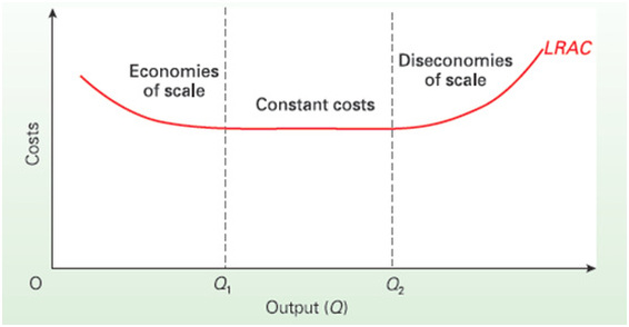
A Typical Long-run Average Cost Curve (Sloman and Wride)
Economies and Diseconomies of Scale
It can be assumed that when a firm expands, it will be able to achieve economies of scale (Sloman and Wride pg 147). Economies of scale occur when an increase in costs and inputs results in a greater increase in output quantity than the increase in costs and inputs (Pilbeam pg 33). The cost per unit is, therefore, lower. It leads to a downward slope of the LRAC curve. Following this downward slope helps illustrate that as you increase output, your production costs per unit decrease.
Up to a point, where the economies are achieved (Q1 above), a doubling in inputs and cost will lead to a doubling in output (Pilbeam pg 34). At a certain point, however, the firm cannot lower the cost per unit of the product anymore. The chart once again illustrates this as the LRAC curve slope gradually flattens.
When the firm gets large enough, production reaches Q2 (above). At this point, managerial and other input related problems might come into play. Here, the firm begins experiencing diseconomies of scale. Now, a doubling in inputs and costs can no longer result in a doubling in output (Pilbeam pg 35). Put differently, when the output increases, production cost per unit also increase. The cost per unit therefore increases when the quantity increases, hence, the LRAC curve slopes upward.
Long Run Marginal Cost
In the long run, the relationship between LRAC and long run marginal cost curves (LRMC) is the same as in the short run (see graph below).
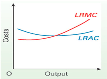
Long Run Average and Long Run Marginal Cost Curves (Sloman and Wride)
Initially, when the firm experiences economies of scale, the additional cost of production of a unit is less than average cost per unit. Hence, the LRMC line is below the LRAC line and the LRAC curve is pulled down. Once there are diseconomies of scale, additional unit of output will cost more than the average. The LRMC curve will be above the LRAC curve and will pull it up (Sloman and Wride pg 147).
Long Run and Short Run Average Costs (SRAC) Relationship
The SRAC curve has a U shaped form. For example, a company with one machine in the short run has the short run average cost illustrated by SRAC1 curve. In the long run, more machines are bought to increase the output. Economies of scale are eventually achieved. With two machines, the average cost of production is shown as SRAC2 curve. In economies of scale, the more machines it has, the lower the SRAC curve and vice versa. The long-run average cost curve can be therefore constructed by enveloping the short run average costs (below).
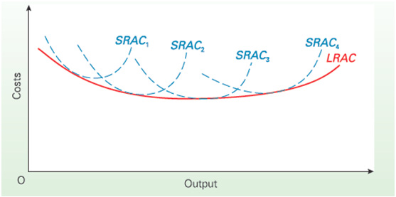
Short Run Average Costs Curves and Long Run Average Cost Curve (Sloman and Wride)
There is a very good video on YouTube that you can find below, which goes through a step-by-step creation of LRAC curve. If you understood what we have written here you can start watching the video from 4:00. If some things are still unclear or if you would like to reinforce the material presented here, you might want to watch it from the beginning.
Works cited for this page
Pilbeam, Keith. 2012 SMM474 Business Economics Lecture presented London: Cass Business School.
Sloman, J. and Wride, A. (2009) Economics. 7th ed. England: Pearson Prentice Hall.
Sloman, J. and Wride, A. (2009) Economics. 7th ed. England: Pearson Prentice Hall.
